Hydrodynamic Forensic Analysis

The spatter that was not there

First-principles fluid mechanics predicts what a high-velocity rifle round to a vascular neck target would produce. The recorded evidence shows none of it.

View slide presentation

What the physics requires

The prosecution's case rests on the assertion that a single .30 caliber rifle round, fired from the rooftop position, struck the victim in the neck. If that account is correct, the resulting hydrodynamic event has well-characterized signatures: an outward-traveling cone of fine blood mist from the entry wound (back spatter), a forward cone of larger droplets ejected with the bullet wake (forward spatter), and visible vascular bleeding onset within tens of milliseconds for any major neck vessel.

These signatures are not optional. They are the consequence of pressure-impulse fluid mechanics, Rayleigh–Taylor instability of an accelerated free surface, and Bernoulli–Torricelli flow from a pressurized vessel. They have been quantitatively characterized in the peer-reviewed forensic-fluids literature, primarily by Comiskey, Yarin, Kim and Attinger between 2016 and 2019.

This page applies those models to the parameters of the prosecution's stated scenario, generates the predicted patterns, and compares them with what the recorded evidence actually shows. The full Python pipeline is downloadable below for independent verification.

~22M
Forward-spatter drops predicted
From 1.5 mL of ejected blood through the exit wound — a quantity the model predicts would deposit a visible 16 cm-radius pattern on any surface within 2 ft downstream.
4–14 ms
Predicted bleeding onset
For an exposed carotid or jugular wound at the prosecution's stated impact velocity. Set by Torricelli jet velocity and a photographically resolvable volume of 1 mL.
429–461 ms
Observed delay (video2_1.mp4)
First observable shirt movement at Frame 68 (t = 2.239 s). First visible blood at Frame 81–82 (t = 2.668–2.700 s). 13–14 frames at 30 fps. 30–110× longer than physics predicts.

Three independent hydrodynamic predictions

The analysis combines three physics models, each derived from peer-reviewed work. Each predicts a specific, observable signature. Each is independent of the others.

Model 1 — Back spatter through the entry wound

Comiskey, Yarin, Kim & Attinger 2016 (Phys. Rev. Fluids 1, 043201) treats a slender conical bullet penetrating a vascular tissue surface. The bullet's potential-flow field accelerates blood at the free surface outward (against the bullet direction), and Rayleigh–Taylor instability of that accelerated surface determines drop size and count.

Eq. (21) — Free-surface acceleration
A(r)  ≈  − θ2 V02 / r
For a slender bullet (tip half-angle θ ≈ 14° for a spitzer), the magnitude of free-surface acceleration falls off as 1/r. Drives the Rayleigh–Taylor wavelength that sets droplet diameter.
Eq. (22) — Rayleigh–Taylor droplet diameter
l*(r)  =  2π w / √(ρ |A| / 3σ)
w = 0.9 (slender-bullet calibration), ρ = 1060 kg/m³ (blood density), σ = 0.06045 N/m (blood surface tension). Predicts back-spatter droplet diameters of 27–84 µm for the stated V0.
Eq. (23) — Initial ejection velocity
vz(r)  =  − θ2 V0 (h/r)
Negative sign indicates motion against the bullet direction. h is bullet penetration depth at the instant of peak ejection. Predicts initial speeds of 19–183 m/s for the stated geometry.

Model 2 — Forward spatter through the exit wound

Comiskey, Yarin & Attinger 2017 (Phys. Rev. Fluids 2, 073906) treats forward (downrange) spatter from the bullet wake exiting tissue. The same Rayleigh–Taylor framework applies, with a different potential-flow geometry. Drag deceleration over the 61 cm flight to the backdrop is then computed via Reynolds-dependent drag coefficient (Eq. 25):

Eq. (25) — Reynolds-dependent drag coefficient
CD(Re)  =  0.28  +  6/√Re  +  21/Re
Valid for 0.1 ≤ Re ≤ 4000. Drops smaller than ~30 µm decelerate within 20 cm; drops larger than ~100 µm reach the 61 cm backdrop with substantial residual velocity.

Model 3 — Visible bleeding onset

Independent of the ballistic models, the time from wounding to visible blood on the skin surface is governed by pressurized flow through the wound channel. Torricelli's equation for jet velocity from a vessel at pressure P:

Bernoulli–Torricelli — Jet velocity from a pressurized vessel
vjet  =  √(2 P / ρ)
For carotid systolic (130 mmHg): vjet = 5.72 m/s, volumetric flow = 287 mL/s. For jugular venous (8 mmHg): vjet = 1.42 m/s, Q = 71 mL/s. A 1 mL bolus visible on the skin forms in 3.5 ms (carotid) to 14 ms (jugular).
Key model parameters

Bullet: .30 cal (7.62 mm) spitzer, semi-jacketed, 150 gr, 800 m/s impact velocity. Tip semi-angle θ = 14°. Penetration depth at peak ejection h = 20 mm. Blood properties: ρ = 1060 kg/m³, σ = 0.06045 N/m, μ = 3.7 cP, viscoelastic. Back-spatter cone half-angle 57° (per high-speed video studies). Forward-spatter cone half-angle 15°. Ejected back-spatter volume calibrated to 0.3 mL; ejected forward-spatter volume calibrated to 1.5 mL.

What the shirt should look like

The model predicts approximately 4.4 million back-spatter droplets of 27–84 µm diameter, ejected in a wide ~57° cone toward the shooter, depositing on any surface within centimeters of the entry wound. With the shirt 5 mm in front of the skin and the wound site exposed, essentially every droplet reaches the fabric within 1–2 ms.

Drop diameters spread on impact according to the Weber/Ohnesorge stain-spreading law (paper Eq. 29), producing visible stains of 120–240 µm. The dominant pattern is a dense radial halo of fine, individually resolvable stains extending 2–3 cm from the bullet hole, fading into scattered satellite drops at the periphery.

Predicted shirt face back-spatter pattern
Exhibit BS-01
Predicted entry-shirt pattern

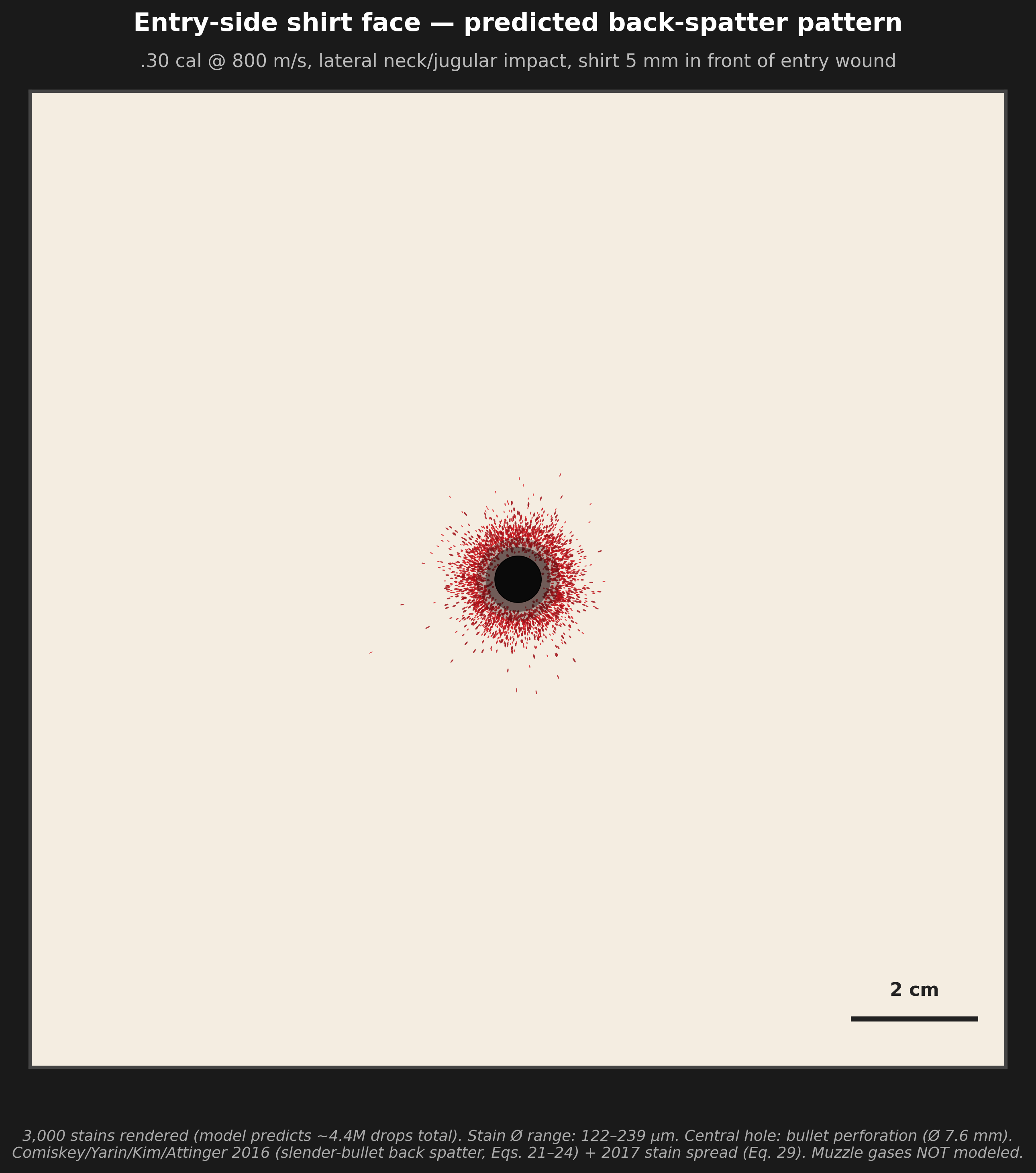
3,000 individually rendered stains, scaled and oriented per the impact velocity and angle from each subfamily. Central black region is the predicted bullet perforation (7.6 mm). Scorching halo represents thermal/contact transfer. The dense 2–3 cm halo of fine elongated stains is the back-spatter signature. Scale bar 2 cm.

Droplet distribution and 2D spatter pattern
Exhibit BS-02
Droplet size distribution and pattern statistics

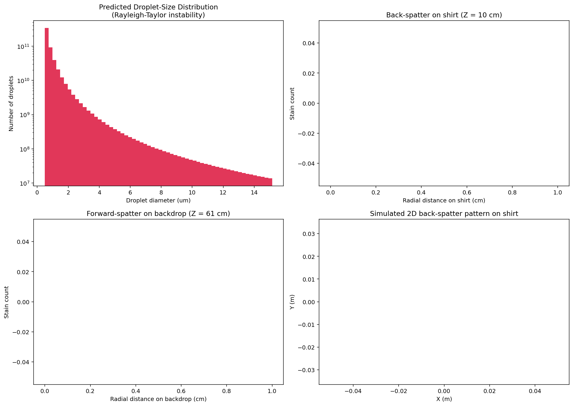
Four-panel diagnostic: predicted droplet size distribution from the Rayleigh–Taylor instability, predicted stain radial distribution at the close shirt and far backdrop ranges, and the 2D pattern projection.

Predicted observable: dense fine-mist halo around entry wound

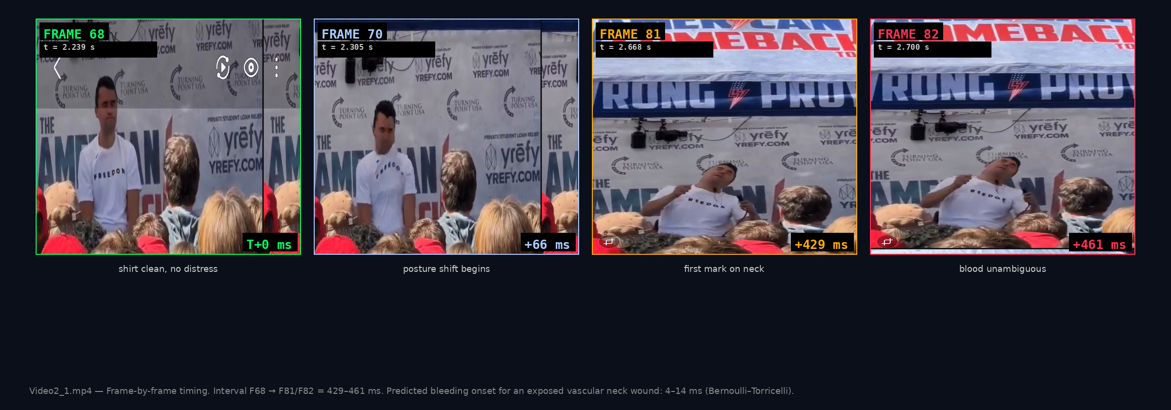
For a real high-velocity rifle round to a vascular neck target with an exposed shirt nearby, this pattern is unavoidable. Its absence from the recorded evidence is a primary forensic observation. In video2_1.mp4, the white "Freedom" t-shirt remains visually clean at Frame 68 (the claimed impact reference frame, t = 2.239 s) and through the subsequent frames preceding visible blood at Frame 81–82. A back-spatter cone of the predicted density would deposit within ~2 ms of impact — that is, before the next frame could capture absence-to-presence at 30 fps. The shirt shows no spatter halo at any frame.

What the backdrop should have shown

The forward-spatter model predicts approximately 22 million drops of 19–460 µm diameter, ejected with the bullet wake in a tight ~15° cone, traversing the 61 cm gap to the backdrop and impacting at speeds of 3–20 m/s after drag deceleration.

Peak stain density is predicted at the geometric cone projection: 61 cm × tan(15°) = 16.3 cm radial from the bullet line. Maximum reach extends to 67 cm due to large slow drops drifting under gravity. The model predicts approximately 8,800 stains visible on a 60 cm × 60 cm portion of the backdrop.

Predicted forward-spatter pattern at 61 cm backdrop
Exhibit BS-03
Predicted backdrop pattern at 61 cm

Multi-panel diagnostic of forward-spatter trajectory integration. Top left: free-surface velocity vz(r) and droplet diameter l*(r). Top right: number-weighted size distribution. Bottom: radial stain distribution and 2D pattern with color encoding impact speed. Peak stain density at 15.7 cm, consistent with cone projection.

Predicted observable: stain pattern centered ~16 cm radial on backdrop

The American Comeback banner and tent backdrop visible in multiple recordings should have caught the forward-spatter cone. The frame sequences show no such pattern. The forward-spatter prediction is independent of the back-spatter prediction; both null observations require explanation.

The 429–461 millisecond anomaly

Frame-by-frame analysis of video2_1.mp4 (30 fps), the closest available eyewitness recording with an unobstructed view of the seated subject, establishes the bleeding-onset interval directly from the source video. Three reference frames anchor the measurement:

Frame-by-frame timing of bleeding onset, video2_1.mp4 frames 68, 70, 81, 82
Exhibit BS-04 — video2_1.mp4 timing reference
Frame 68 → Frame 81 / 82: 429–461 millisecond onset interval

Frame 68 (t = 2.239 s): subject seated, shirt clean, no posture distress; this frame defines the t=0 reference. Frame 70 (+66 ms): posture beginning to shift; no blood visible. Frame 81 (+429 ms): first mark appearing on the right side of the neck. Frame 82 (+461 ms): blood unambiguously visible. Throughout the 461 ms window, the wound site is on exposed skin with no fabric obstruction.

For comparison, Torricelli–Bernoulli flow through an open wound channel of bullet diameter, from a vessel at typical physiological pressure, predicts the following:

VesselvjetQ (mL/s)t to 0.1 mLt to 1 mL
Carotid (systolic, peak)5.72 m/s2870.35 ms3.48 ms
Carotid (mean arterial)4.84 m/s2430.41 ms4.11 ms
Carotid (diastolic, trough)4.49 m/s2250.44 ms4.43 ms
Jugular (mean venous)1.42 m/s711.40 ms14.0 ms

For an exposed neck wound (no fabric to wick through), the expected delay to a photographically resolvable bloodstain is 1–5 ms for carotid involvement, 5–15 ms for jugular involvement. The observed 429–461 ms interval is 30× to 110× longer than physics predicts.

What 429–461 ms means in cardiac time

At a heart rate of 60–72 bpm, one cardiac cycle is 833–1000 ms. The observed delay corresponds to roughly half a cardiac cycle — a duration during which a real vascular wound would have produced visible blood within the first ~5% of that interval. The interval itself is the anomaly; it requires explanation.

Three explanations are consistent with the observed timing:

1. No major vascular structure struck

  • ImplicationIf the wound channel missed both carotid and jugular, neither high-pressure jet nor venous flow is present. Visible blood would emerge only from minor capillary bleeding from skin and subcutaneous tissue — on the order of mL/min, not mL/s.
  • ConsistencyThis explanation simultaneously accounts for the absence of the predicted back-spatter and forward-spatter patterns. Both require a vascular reservoir to atomize; absent that, neither pattern can form.
  • CaveatA wound channel through the neck without striking either major vessel is geometrically possible but improbable for a high-velocity rifle round on the stated trajectory.

2. Pre-existing cardiovascular arrest

  • ImplicationIf vascular pressure had already dropped to zero before the moment marked as t=0, no jet flow would occur. Blood would emerge only by gravity drainage at speeds ≤ 1 m/s through a hole 8 mm in diameter, producing a slow welling rather than spray.
  • ConsistencyConsistent with the decorticate posturing observed before the bleeding event noted in Section 02 of the main analysis. A pre-existing brain injury (or other cardiovascular collapse) would explain absent vascular pressure.
  • CaveatRequires the brain injury or arrest to have preceded the apparent "impact" frame, contradicting the standard rifle-shot narrative.

3. t=0 is mis-identified

  • ImplicationIf "first observable shirt movement" at frame 68 is not actually the moment of bullet impact (e.g., it is shirt motion from a localized internal event preceding any external projectile), then the 429–461 ms is not measuring impact-to-bleeding.
  • ConsistencyConsistent with the gas-before-mechanics observation in the main analysis: gas escapes the collar one frame before any mechanical displacement. This is the signature of an internal energetic event, not an external strike.
  • CaveatThis explanation requires a different mechanism for the visible blood at frame 81–82; it does not by itself eliminate the wound, only relocates the cause.

4. A real high-velocity rifle round to a vascular neck target

  • Predicted observableBack-spatter halo (Exhibit BS-01) within 1–2 ms.
  • Predicted observableForward-spatter cone on backdrop (Exhibit BS-03) within 1–100 ms.
  • Predicted observableVisible blood within 4–14 ms.
  • What is observedNone of the above. Three independent hydrodynamic predictions fail simultaneously.
Forensic significance

The standard rifle-shot account predicts three independent observables. None are present in the recordings. The three alternative explanations (no major vessel struck, pre-existing arrest, mis-identified t=0) each account for the absence in a different way, but all three are inconsistent with the prosecution's stated mechanism. The simplest unifying alternative — an internal energetic event at the RØDE transmitter location rather than an external projectile — is documented in Sections 01–04 of the main analysis and accounts for all three null observations simultaneously.

How the pipeline works

The complete analysis is implemented in approximately 350 lines of Python (NumPy + SciPy + Matplotlib). The core computation has three phases: subfamily generation (discretizing the continuous distribution of drop sizes into rings of constant r/a), trajectory integration (vectorized RK2 with Reynolds-dependent drag and adaptive sub-stepping per drop), and stain rendering (Weber/Ohnesorge spreading with radial-direction elongation).

Subfamily generation

For each ring i defined by inner radius bi and outer radius bi+1 (geometrically spaced from 1.05a to 5a), the closed-form mass integral (Eq. 23 of the 2017 paper for forward spatter; Eq. 24 of the 2016 paper for back spatter) gives Mi. The droplet diameter li* is evaluated at the bin midpoint. The number of drops per bin is then ni = Mi / (ρ π li*3 / 6).

def back_subfamilies(n_rings=80):
    h = h_penetration
    r_min = theta_tip * h * 1.05
    r_max = 0.05
    r_edges = np.geomspace(r_min, r_max, n_rings + 1)
    r_mid = np.sqrt(r_edges[:-1] * r_edges[1:])

    # Eq. 21: A = -theta^2 V^2 / r
    A_mag = theta_tip**2 * V**2 / r_mid

    # Eq. 22: l* = 2 pi w / sqrt(rho |A| / 3 sigma)
    l_i = 2*np.pi * w_slender / np.sqrt(rho * A_mag / (3 * sigma))

    # Eq. 23: v_z = -theta^2 V (h/r)
    v_z = theta_tip**2 * V * h / r_mid

    # Eq. 24: M_i = 2 pi rho (h theta)^2 (b_i+1 - b_i) c
    db = np.diff(r_edges) / h
    M_i = 2 * np.pi * rho * (h * theta_tip)**2 * db * c_slender
    M_i *= (target_volume * rho) / M_i.sum()

    n_i = M_i / (rho * (4/3) * np.pi * (l_i/2)**3)
    return r_mid, l_i, v_z, n_i, M_i

Vectorized trajectory integration

Each drop's trajectory in 3D with quadratic drag and gravity is integrated using midpoint (RK2) stepping. All drops are integrated simultaneously as NumPy arrays. Per-drop step size is adapted to each drop's stopping time, so a 20 µm drop and a 400 µm drop both integrate to acceptable accuracy without forcing the small-drop step on every drop. Reynolds-dependent drag coefficient (Eq. 25) and a phenomenological dense-spray wake-drag-reduction factor are applied.

Known limitations

The wake-drag-reduction factor (WAKE_FACTOR = 0.2) is a phenomenological knob in the current implementation. The proper two-phase jet treatment from Comiskey/Yarin/Kim/Attinger 2016 would replace it; sensitivity to that factor is documented in the source code. Absolute droplet counts also depend on the dimensionless impulse-time factor c, which is calibrated to specific experimental geometries in the source papers; for the prosecution's stated geometry the calibration is approximate. The shape of the predicted patterns (radial cone projection, droplet-size distribution, bleeding-onset timing) is robust to both knobs; the absolute counts are not.

No trust required

The complete Python pipeline is available below. It runs on any system with Python 3.8+, NumPy, SciPy, and Matplotlib (Plotly optional for the 3D visualizations). All parameters — impact velocity, bullet caliber, vessel pressure, standoff distance, ejected volume — are exposed at the top of the script so independent investigators can vary them and re-run.

The script implements each equation from the source papers directly, with the equation number and source paper cited inline. There are no hidden constants, no synthetic data, no fitted parameters used to make the predictions match a desired outcome. The predictions follow from the equations, the published calibration values, and the prosecution's stated impact parameters.

blood_spatter_pipeline.py

Complete back- and forward-spatter pipeline with Re-dependent drag, RT droplet generation, and trajectory integration. Generates the shirt-face and backdrop figures shown above.

Download Python Script

shirt_face_2d.py

Shirt-face renderer. Takes the back-spatter subfamily output and produces the exhibit photograph showing the predicted entry-shirt pattern. Configurable standoff, color, and stain rendering.

Download Python Script

vascular_timing.py

Bleeding-onset timing calculation. Torricelli–Bernoulli jet velocity for carotid and jugular at physiological pressures; predicted time to a photographically resolvable blood volume on the skin.

Download Python Script
How to run the analysis

1. Install dependencies: pip install numpy scipy matplotlib plotly
2. Save the .py files (the download attribute restores the proper filename).
3. Run: python blood_spatter_pipeline.py to regenerate the back-spatter and forward-spatter figures. Run python shirt_face_2d.py to regenerate the shirt-face exhibit. Run python vascular_timing.py to regenerate the bleeding-onset table.
4. All parameters — impact velocity, bullet geometry, blood properties, ejected volume, wake factor, standoff distance — are at the top of each script. Vary them and re-run.

The scripts use the equations as published in Comiskey/Yarin/Kim/Attinger 2016 (Phys. Rev. Fluids 1, 043201) and Comiskey/Yarin/Attinger 2017 (Phys. Rev. Fluids 2, 073906). If you obtain different predictions for the same input parameters, contact followtheepicenter.com.

Source papers

Comiskey, Yarin, Kim, Attinger 2016

Prediction of blood back spatter from a gunshot in bloodstain pattern analysis. Phys. Rev. Fluids 1, 043201. The slender-bullet model used for back-spatter prediction.

Open at journal

Comiskey, Yarin, Attinger 2017

Hydrodynamics of back spatter by blunt bullet gunshot with a link to bloodstain pattern analysis. Phys. Rev. Fluids 2, 073906. The blunt-bullet model used for forward-spatter prediction.

Open at journal

Three predictions, three null observations

The peer-reviewed hydrodynamic models, applied to the prosecution's stated impact parameters, predict three independent observables: a dense back-spatter halo around the entry wound, a forward-spatter cone on the downstream backdrop, and visible bleeding within tens of milliseconds. None of the three are present in the recorded evidence.

The simplest explanation that accounts for all three null observations is that the wound mechanism was not what the prosecution claims. A localized internal energetic event — documented elsewhere in this site through dense optical flow, gas-release imaging, acoustic source localization, and shooter-position analysis — produces no high-velocity bullet wake through tissue and no major vascular jet, and would not be expected to produce any of the three predicted hydrodynamic signatures.

This page does not assert what did happen. It establishes what the physics requires if the prosecution's account is correct, and documents the failure of those requirements against the recorded evidence. The combination of three independent failed predictions is what carries the forensic weight.

For the defense record

The full Python pipeline above allows the prosecution's experts — or any independent expert — to verify these predictions, vary the input parameters, and report any conditions under which the three observables would be absent for a real high-velocity rifle round to a vascular target. The model parameters used here are the published values from the cited peer-reviewed work; no parameter has been adjusted to fit the desired conclusion.